Jev (System One) sub-calls for Recursive Language Models

tl;dr

Recursive Language Models (RLMs) let a root LM work through contexts far bigger than its window. The context lives in a REPL variable, and the root writes code over it and calls sub-models on pieces of it. On aggregation tasks most of those sub-calls are judgments (label this line, is this passage relevant), so this weekend I started exploring what happens when you hand them to Jev, TypeSafe’s “System One” model, which returns calibrated probabilities instead of text, to get a feel for where it’s useful.

As a sub-call, Jev is about as accurate as Claude Haiku 5.5 (93.6% vs 92.0% with thinking off, 95.0% with it on) and several times faster. Inside an RLM the two scored the same on OOLONG from 32k to 1M tokens, but at 1M the Jev RLM cost half as much and ran six times faster. The bigger difference is what comes back. Roots used the probabilities without being asked, for expected counts, cross-checks and inspecting borderline items, and the same probabilities let a program skip its least confident answers (0.79 → 0.92 on OOLONG) or send only uncertain items to a bigger model, which beat both models alone (at the best threshold, chosen after the fact).

One practical rule: never make Jev find items by position. Asking about records[17] in an unlabeled list fell from 94% to 26% accuracy at 250 items per request; putting each item in its own question held 95%.

The long-context results re-confirm the RLM paper on Claude. At 131k the Jev RLM scored 0.66 against 0.53 for Sonnet 5.5 reading everything, and on OOLONG’s 1M contexts, which are just over Sonnet’s window, 0.70 against 0.40 truncated. One result went the other way. On BrowseComp-Plus the root did as well with plain regex as with Jev, and 7× faster.

I’ve packaged the tools as rlm-jev; they plug into dspy.RLM or Alex Zhang’s rlm library. All the raw results and the scripts that produce them are in the repo.

Code: github.com/jhochenbaum/rlm-jev · Every number in this post: results/summary.json

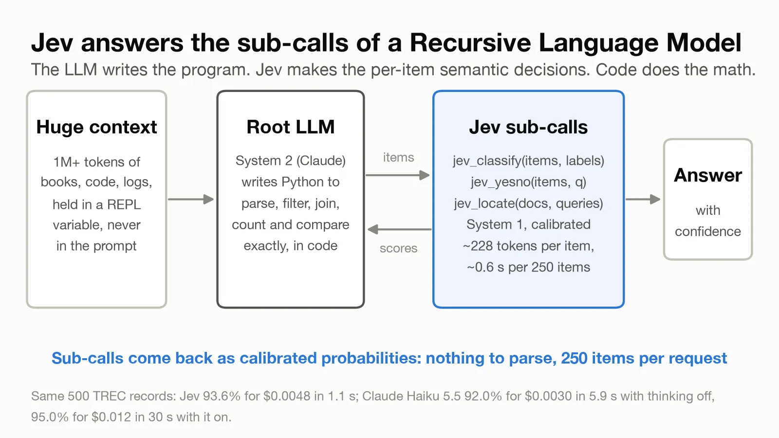
On aggregation tasks, RLM sub-calls are mostly decisions

Alex and Omar introduced RLMs in a blog post, followed by a paper with Tim Kraska. Their argument is that a long context is better treated as an environment the model programs against than as a prompt it has to read. The root LM sees the question and a handle to the context, and decides for itself what to look at and what to hand off. With GPT-5 as the root, that beat reading the whole prompt, and the usual long-context scaffolds, on four benchmarks, and kept working on inputs about 100× larger than the model’s window.

This post builds directly on that work. I use their benchmarks: OOLONG at 131k and 1M tokens, the OOLONG-Pairs variant they built, and BrowseComp-Plus in the paper’s 1,000-document setting. I also use their depth-1 setup, and adapt the truncated-read baseline Alex used on BrowseComp-Plus. The main thing I change is what a sub-call returns.

Their post also describes the strategies their root LM fell into, among them peeking, grepping, partition + map, and summarization. On aggregation benchmarks like OOLONG, partition + map does most of the work. The root chunks the context, asks a sub-LM to label each question in the chunk, and then answers from the labels. In their example the sub-LM is GPT-5-mini, and its primary job is reading a few hundred lines and writing back a category for each one.

Small LLMs have gotten pretty good at this kind of classification (Haiku 5.5 gets 95% on the items later in this post), but generating text was never really the natural interface for it. The root wants one label, or one yes/no, per item. The sub-LM writes them out token by token as prose or a numbered list, the root parses that, and it has to handle the times it doesn’t parse. Whatever the sub-LM knew about its confidence in each item is lost along the way. The root gets back a string when what it really wanted was a label and a confidence.

In September TypeSafe released Jev, the first of what they call System One models, after Kahneman’s fast, intuitive System 1. Jev doesn’t generate text. In TypeSafe’s words, it “evaluates typed questions against a state and returns structured results directly.” You send it a state (some text) and a set of typed questions, and it returns a probability for every possible answer:

state = "Hi, my payouts have failed for 3 days and I'm losing sales."
questions = {
    "urgent": Noul("Does this message convey urgency?"),  # yes/no
    "department": Choice(                                  # pick one
        "Which team should handle it?",
        {"billing": "...", "technical": "...", "sales": "..."},
    ),
}
# -> {"urgent": 0.95,
#     "department": {"technical": 0.85, "billing": 0.15, "sales": 0.0}}

Noul is TypeSafe’s name for a yes/no question. The probabilities are trained to be calibrated, meaning that when Jev says 0.8, it should be right about 80% of the time, and on my items the calibration error was 0.02. It costs $0.042 per million input tokens, output is free (pricing), and a request carrying 250 questions came back in about 0.6 seconds.

That makes Jev close to what a programmer would want a sub-call to be: a function with a typed signature that returns a distribution. Alex has pointed at Jev as the kind of non-autoregressive tradeoff that fits RLMs. I wanted to see whether that holds up on the benchmarks RLMs are measured on.

The setup

As in the RLM paper’s default setting, everything here is depth 1, meaning the root calls plain models, not other RLMs. It gets these functions:

• jev_classify(items, labels) returns a distribution over the labels for each item.
• jev_yesno(items, question) returns P(yes) for each item.
• jev_locate(docs, queries) scores passages against queries (see “Finding a passage without an index” below).
• jev_spend() reports spend against a dollar cap, which the tools enforce.

Each call packs hundreds of items into one request and runs requests concurrently. Otherwise the root is an ordinary RLM root, and in dspy.RLM it keeps its LLM sub-call (llm_query) for anything that needs text back:

import dspy
from rlm_jev import rlm_tools

dspy.configure(lm=dspy.LM("anthropic/claude-sonnet-5-5"))
rlm = dspy.RLM("context, query -> answer", tools=rlm_tools(max_usd=0.50))
rlm(context=huge_text, query="Which user posted the most spam?")

Here is a full root trajectory on an OOLONG question, is the label “location” more or less common than “entity”?, over 787 lines. It takes three turns (label descriptions trimmed):

# turn 0: peek at the head and the tail
lines = context.split("\n")
print(context[:1200]); print(lines[-5:])
# turn 1: pull out the questions, dedupe, one bulk call, count in code
pat = r"Date: .*? \|\| User: \d+ \|\| Instance: (.*)"
items = [m.group(1) for l in lines if (m := re.match(pat, l))]
labels = {
    'location': 'answer is a place, such as a country, city, mountain, ...',
    'entity': 'answer is a thing, animal, object, food, product, '
              'creative work, event, ...',
    ...
}
uniq = list(dict.fromkeys(items))
res = jev_classify(
    uniq, labels,
    instruction="What category does the answer to this question belong to?",
)
mp = dict(zip(uniq, res))
c = Counter(max(mp[i], key=mp[i].get) for i in items)
# Counter({'entity': 183, 'human being': 146, 'abbreviation': 124, ...,
#          'location': 98})
# turn 2
FINAL("Answer: location is less common than entity")

Partition + map collapses into a single call here, since with 250 items per request there’s nothing to gain from chunking.

Batching hundreds of items per request

Jev bills the state once per request, and each extra question adds only its own text and a few tokens of structure, so it pays to ask about many items at once. My first layout got that wrong. I put a batch of records into the state as a plain list and asked one question per record: “which category is records[17]?” With one record per request, accuracy was 94%. With 25 it was 88%, with 100 it was 34%, and with 250 it was 26%.

The problem was the addressing, not the state. Nothing in the list marked which record was number 17, so Jev had to count positions, which models in general do badly. When I gave each record a visible ID in the state (r17: ...) and asked about r17, accuracy held at 95–97% all the way to 250 records per request. Putting each record inside its own question instead, with the state holding only shared context like the task description, did just as well, 95% at 250 per request.

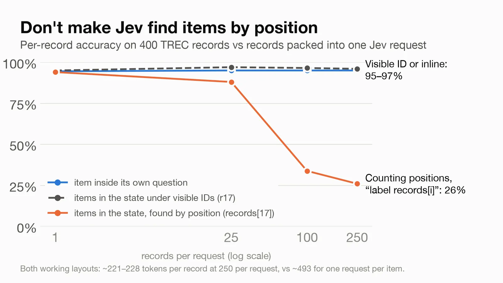
Both working layouts cost about 221–228 tokens per record at 250 per request. One request per record costs 493 tokens (DSPy’s built-in Jev integration works this way and uses 514), so batching roughly halves the tokens and needs 1/250th of the requests. The request count turned out to matter, because under load I hit throttling and timeouts well below the documented 80 requests per second.

Shared text can go in the state too, with a trade-off. In these runs each question carried the six label descriptions, about 200 tokens paid 250 times per request. Writing them once in the state and giving each question only the label names cut the cost to 89 tokens per record, 2.6× less, with the same calibration. But on all 4,151 TREC records accuracy fell from 94.4% to 92.8% (both option orders averaged), and the per-label counts drifted further from the truth (11% error against 8%). Dropping the descriptions altogether cost 13 points. Everything below uses the descriptions-in-every-question format, which is also rlm-jev’s default; the shared format is an option, and the six-weight correction later in the post works especially well with it.

How the roots used Jev

I read through 127 OOLONG transcripts looking for patterns that come from having a decision model as the sub-call.

Every root peeks at the head of the context within its first three turns, and most (101 of 127) also print the tail, because OOLONG’s footer repeats the label set. It reminded me of a programmer opening an unfamiliar file.

49 of the 58 runs that call jev_classify deduplicate first and multiply the counts back with a Counter, without being told to. At 4M tokens this turns 102,158 lines into 4,151 unique questions, cutting the cost 24.6×. Two roots went further. They noticed that about 80 acronym questions (“What is DTMF ?”) each repeat 62 to 65 times, so a single unstable label moves a count by 60. One of them reworded its label descriptions and watched the abbreviation count move from 5,010 to 4,166.

Most roots take the argmax, but a fair number use the probabilities directly. About 14 runs sum them into expected counts, weighted by how often each question repeats:

soft[k] += v * mult[u]          # expected count, not argmax count

About 13 list borderline items (top probability under 0.6, or a runner-up above 0.2) and inspect them. Nineteen cross-check jev_classify with a jev_yesno question, and one of them averages the two and flags whatever is still in doubt:

comb = {q: (probs[q] + ynd[q]) / 2 for q in uq}
border = [q for q in uq if 0.3 < comb[q] < 0.7]

With a generative model in the sub-call, the root would only have the labels to work with.

In 9 of 67 runs the root never calls Jev. Three are “which user posted most” questions, which a Counter answers directly. The other six ask about a single user’s 9 to 16 lines, and the root reads and labels them itself.

The Haiku arm shows where generative sub-calls cause trouble. At 32k the root sends batches of 50 questions and parses N: label lines back with a regex. In 5 of 15 batched runs the first pass came back incomplete (760 to 786 of 787 labeled). Two roots noticed and re-asked; three carried on with up to 19 items missing. One got a truncated label back for 42 items. Jev returns one distribution per question every time, so the root never has to parse a reply.

Results

All runs use a Claude Sonnet 5.5 root. The LLM sub-call baseline is Claude Haiku 5.5, run through the Claude Code CLI, which keeps Haiku’s extended thinking on (it can’t be turned off there). The one comparison with thinking off went through the Anthropic API. Claude costs are list prices for the same token counts as API calls, with prompt-cache writes at the 5-minute rate. I report two kinds of result:

• Live runs are the real RLM, where the root reads the question and writes its own program.
• Fixed-program runs use the same program every time: it labels every line with the sub-call model and computes the answer in code, which measures the sub-call model on its own. The program scores 1.0 when fed the true labels, so any gap below 1.0 comes from the sub-call model.

OOLONG scores use the benchmark’s own metric, with exact match for labels and comparisons and partial credit for counts that are close.

Jev vs Haiku as the sub-call model

To isolate the sub-call model, I took 500 questions from the slice of TREC that OOLONG is built on and had each model assign the same six categories. Jev got 93.6% in a single pass for $0.0048, in 1.1 seconds. Claude Haiku 5.5 through the API with thinking off got 92.0% for $0.0030 in 5.9 seconds. That’s a little cheaper than Jev, a little less accurate, and five times slower. With the label descriptions sent once per request (see Batching), Jev costs $0.0019 for the same 500, but is about 1.5 points less accurate across all 4,151 TREC records (92.8% vs 94.4%). (Through the CLI with thinking on, as in the RLM runs, Haiku got 95.0% for $0.012 in 30 seconds, including CLI startup for each call.)

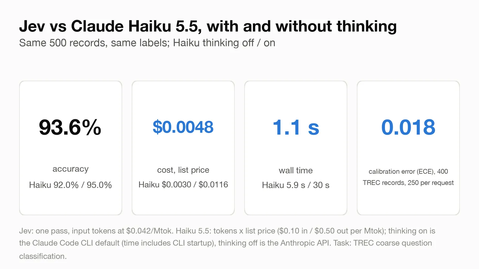
These items are easier than TREC as a whole. On the 490 TREC test questions outside OOLONG’s slice Jev scores 90.8%, and on 1,000 of the 1,721 TREC questions OOLONG left out it scores 72%. Those are harder for Haiku too (78% with thinking off), but Jev falls further, trailing Haiku by about 6 points there, where it was a point ahead on OOLONG’s slice.

In full RLM runs on 20 OOLONG questions at 32k tokens:

Setup (n = 20)	Score	Cost / q	Time / q
Sonnet 5.5 reads the whole context (no RLM)	0.76	$0.17	49 s
Haiku 5.5 reads the whole context (no RLM)	0.54	$0.006	19 s
RLM, Haiku 5.5 sub-calls	0.72	$0.073	57 s
RLM, Jev sub-calls	0.68	$0.071	34 s

At 32k it’s best to just read the context with Sonnet, since it fits easily in the window and the direct read scores highest. Haiku reading the same context is far cheaper but scores 0.54. The two RLMs cost the same, because with sub-calls this cheap the root is most of the bill (about 86% of it with Jev). The Jev RLM is faster, since one bulk call replaces about fifteen generative ones. The score differences are within noise at n = 20. At short contexts, then, the choice of sub-call model makes little difference.

OOLONG from 32k to 4M tokens

OOLONG asks aggregate questions over thousands of lines: which label is most common, how many lines from these users are spam, did this label get more or less common after a given date. Every line needs a semantic judgment, and the answer needs exact arithmetic over all of them, so retrieving a few relevant lines doesn’t help.

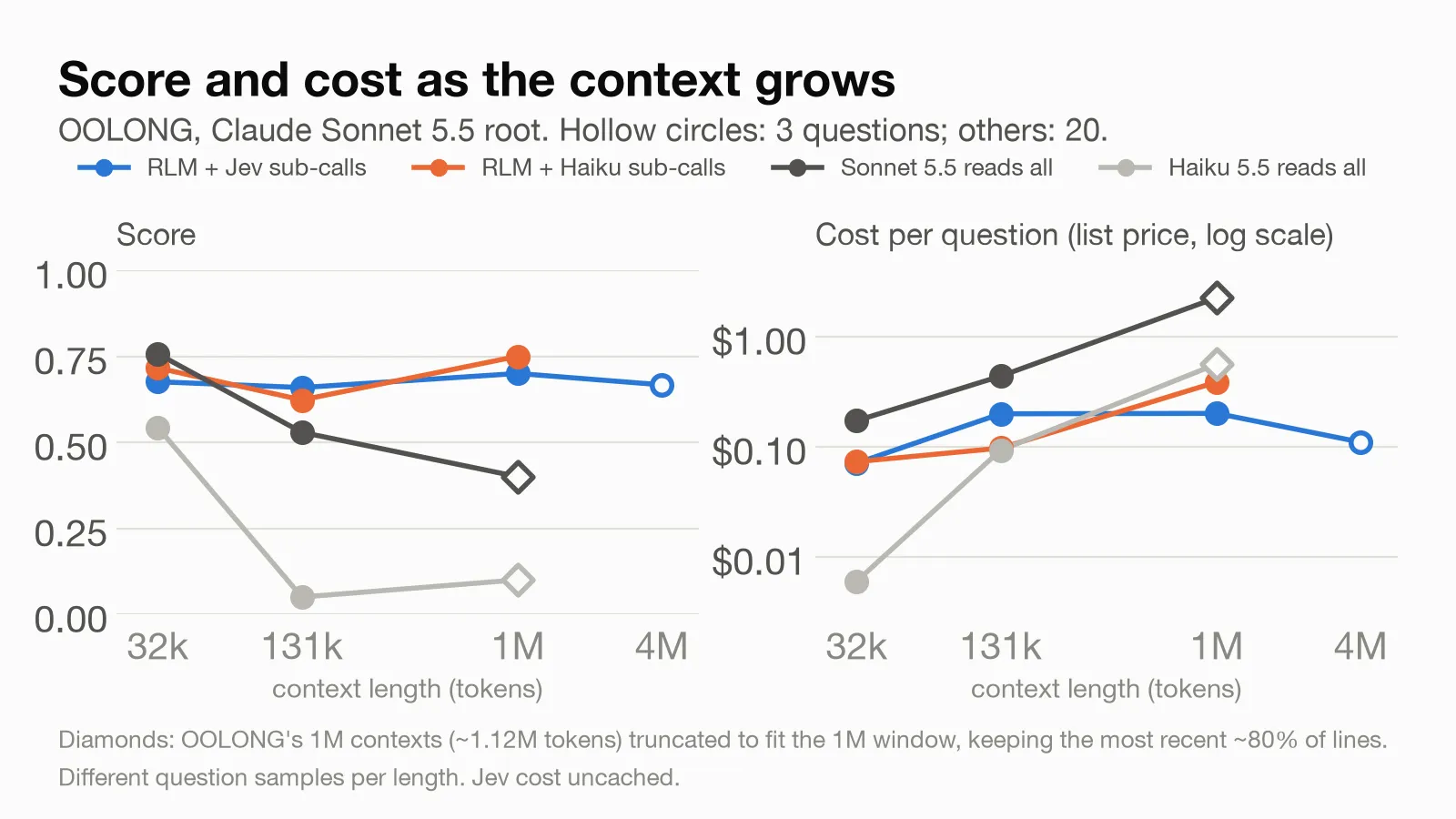
Sonnet 5.5 reading the whole context falls from 0.76 at 32k to 0.53 at 131k, at $0.44 a question, and Haiku 5.5 falls harder, from 0.54 to 0.05. OOLONG’s “1M” contexts are about 1.12M tokens, just over both models’ windows, so for those I adapted the RLM post’s truncated baseline, keeping the task header and the most recent ~80% of the lines. Truncated, Sonnet scored 0.40 at $2.25 a question and Haiku 0.10. A perfect reader of the kept lines would still score 0.75, so most of Sonnet’s loss comes from reading rather than truncation.

The RLM with Jev sub-calls scored 0.66 at 131k, 0.70 at 1M (20 questions each) and 0.67 at 4M (3 questions), for about $0.20 a question or less. With Haiku sub-calls it scored 0.62 and 0.75, a tie at these sample sizes. At 131k the Haiku RLM was cheaper ($0.10 a question), mostly because its roots took fewer turns. At 1M it needed about 144 sub-calls a question, so it cost twice as much and took six times as long. The question samples differ by length, so the curve shows the RLM holding up where reading everything degrades; it doesn’t show the RLM improving with length.

Cost stays roughly flat because the root deduplicated before calling Jev, and OOLONG’s long contexts repeat questions heavily. At 1M, 25,531 lines became 4,151 unique questions; at 4M, 102,158 lines became the same 4,151. Labeling those costs about four cents, and the whole 4M question cost $0.11.

The hardest variant, OOLONG-Pairs, asks for every pair of users who satisfy a condition on both, so the work grows with the square of the number of users. Inside an RLM it reduces to labeling every line once and doing the join in code. F1, a 0-to-1 score for how well the returned pairs match the true set, was 0.77 with the root writing that program live (4 questions), and 0.85 at 32k and 0.89 at 131k with the fixed program. The RLM paper reports essentially zero for base GPT-5 and 0.58 to 0.76 for its GPT-5 RLM. Those runs used different root and sub-call models, so the numbers aren’t directly comparable.

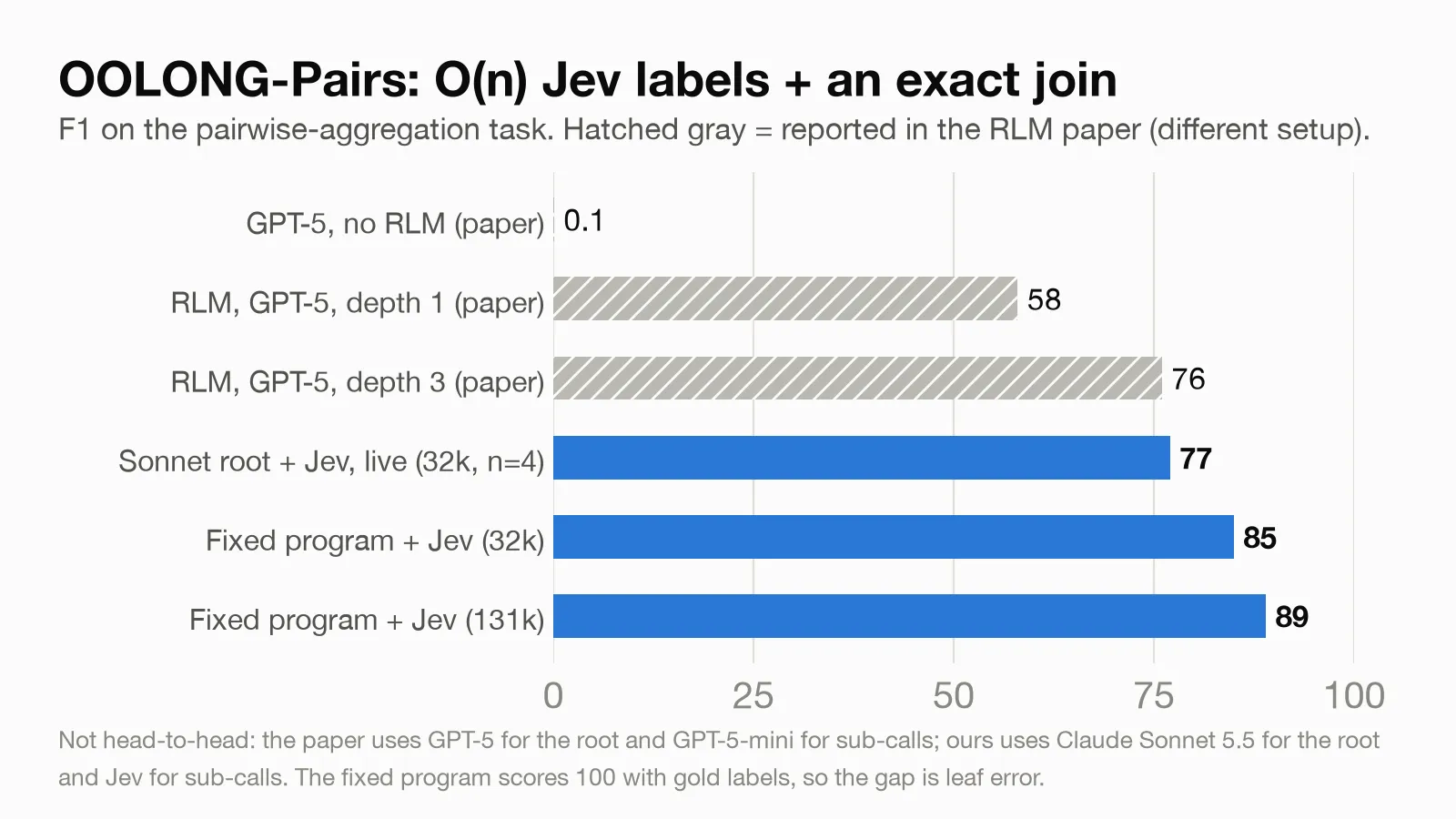
To check that I hadn’t tuned to the data I’d been looking at, I ran the fixed program on the OOLONG test split at 131k, which covers 8 datasets I never looked at while building this. With no tuning beyond the label names in each dataset’s header, it scored 0.79. Always guessing the most common label scores 0.46.

Finding a passage without an index

Some long-context questions aren’t aggregation. The root needs the one passage that answers something, and the passage is worded nothing like the question. The RLM post points out that indexing a retriever on the fly is expensive, which is why its roots grep instead. Grep only works when you know the words. jev_locate is a semantic grep over whatever text is in a variable.

It works in two passes. The first splits the corpus into windows of about 1,500 words and sends each window once as the state, with every query attached as its own yes/no question, so all the queries share a single read of the corpus. The second pass scores the lines inside the best windows.

To test it, a separate agent wrote 30 facts and 30 questions with no content words in common (the fact says “apothecary,” the question says “chemist”), and the facts were hidden in 1.2M tokens of 19th-century novels. I compared Jev against the standard open retrieval pipeline at three sizes: a Qwen3 embedding model fetches the top 100 sentences by vector similarity, then a Qwen3 reranker re-scores those 100.

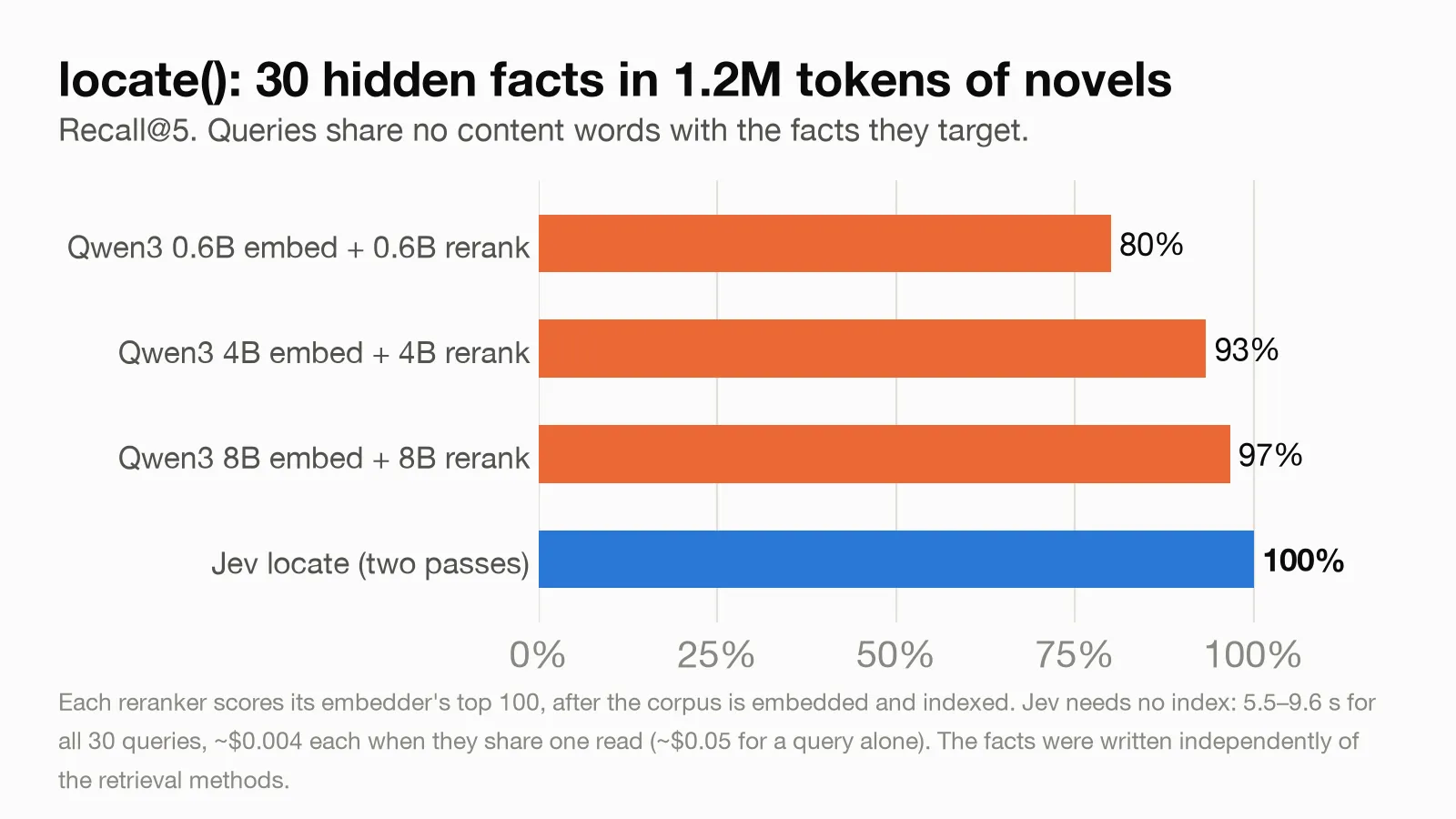
Jev put all 30 facts in its top five, 28 of them at rank 1. The Qwen3 pipeline found 80% at 0.6B, 93% at 4B and 97% at 8B (29 of 30, 26 at rank 1). Each query found its own fact rather than one of the other 29 planted sentences, so all of these systems were matching meaning rather than spotting out-of-place text.

On accuracy, a strong 8B retrieval stack is about as good as Jev here; one fact out of 30 is noise. But on any meaningful corpus, the embedding pipeline needs GPUs and an index built ahead of time. Once that’s built it answers new queries fast, so for a fixed corpus that gets searched a lot it’s the better tool. Jev needs no index or setup and reads whatever text the root is holding. A single query costs about $0.05, almost all of it the window pass over 1.2M tokens; queries asked together share that pass, so these 30 came to about $0.004 each. The window pass took 5.5 seconds, and 9.6 with the line pass. It also returns calibrated probabilities the root can threshold. Inside an RLM, where the context is different for every task, I think that trade usually favors Jev.

I also tried Jev as a front end for a reader model. On InfiniteBench’s multiple-choice questions about whole novels, Jev picked about 8,000 words of evidence and Haiku 5.5 answered from those. The alternative was Haiku 5.5 reading the entire book, which its 1M-token window now allows for most of them:

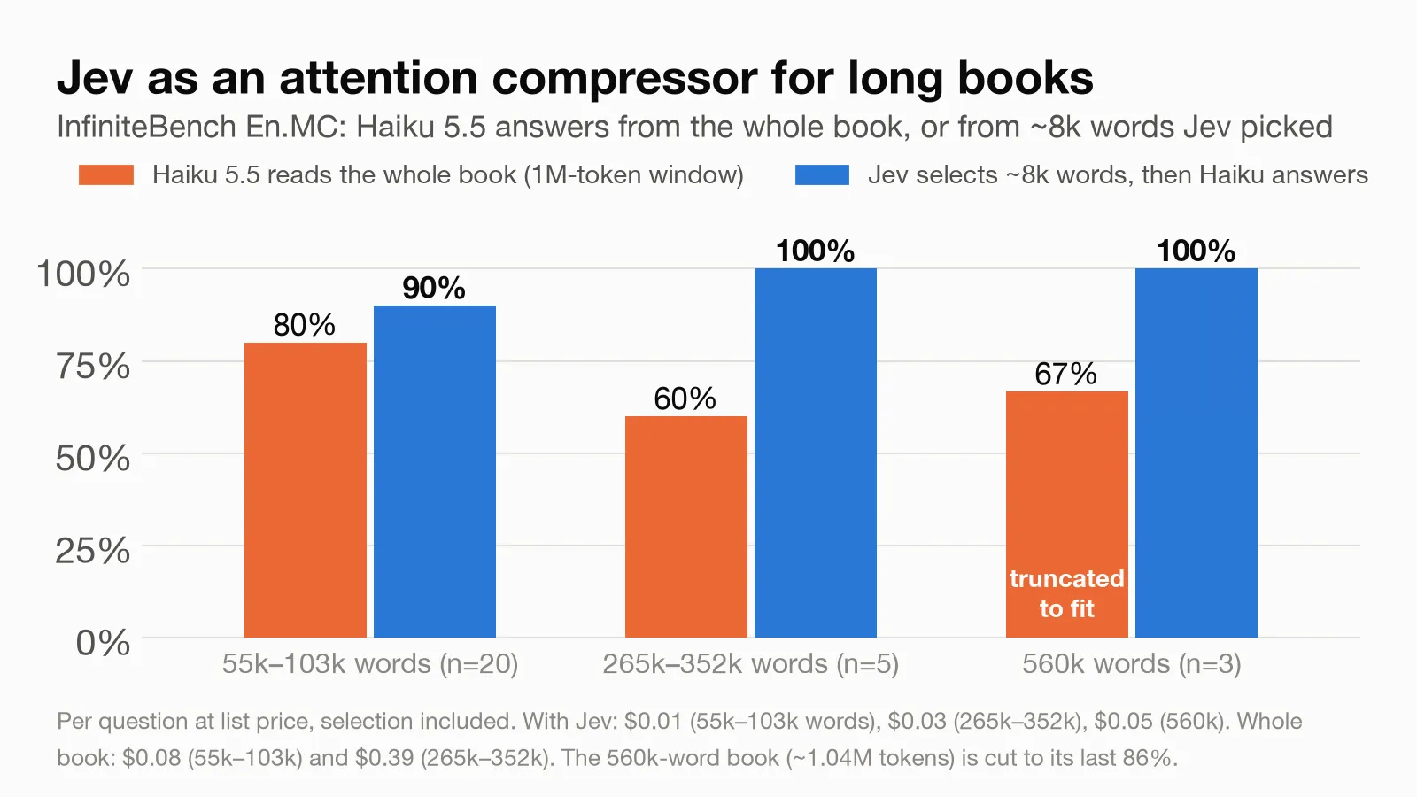
Reading only Jev’s selection did better at every length. On books of 55k to 103k words it scored 90% against 80% for the whole book (20 questions), and on books of 265k to 352k words, all inside the window, 5 of 5 against 3 of 5. The longest book, 560k words, doesn’t fit; Jev’s selection answered all 3 of its questions, and Haiku reading a truncated copy answered 2. A question cost $0.01 to $0.05 with Jev against $0.08 to $0.39 for the whole book, but the selection was slow at this scale, from about 80 seconds a question on the shorter books to 5 to 10 minutes on the longest. The samples are small, but they agree with the 131k OOLONG result that a context that fits in the window still isn’t necessarily read well.

BrowseComp-Plus

BrowseComp-Plus is the RLM paper’s flagship benchmark. It asks hard research questions that need several linked facts, over 1,000 web documents per question (about 8M tokens), with the documents needed to answer guaranteed to be among them. The root gets jev_scout, which scores each document’s opening; jev_search, which scores every window against all of its queries at once; and read, which returns text. It can also run any Python over the docs list.

On 20 questions (the paper used 150), the RLM answered 18 correctly (90%) with a 30-turn limit, and 17 (85%) with 14 turns. The paper’s GPT-5 RLM scored 91% on its 150. Eleven of the 18 matched the reference answer exactly; Claude Sonnet 5.5 judged the other seven correct (majority of three votes).

Asked the same questions with no documents and no tools, Sonnet 5.5 got 2 of 20. The RLM got both of those right too, plus 16 more, so its answers came from the documents. Then I removed the Jev tools and ran the 20 questions again. The root scored 18 of 20 with regex alone, in about 2 minutes a question instead of 14, for $0.31 of Sonnet, against $0.24 of Sonnet plus $0.03 of Jev.

In the transcripts, the roots with Jev used jev_scout to rank documents by their openings, then switched to regex over the full documents for the specific clues. Counting occurrences in the roots’ code, jev_scout appears about 4 times a question and re.search about 8, and jev_search once in 20 questions. Without Jev, re.search appears about 14 times a question. BrowseComp-Plus clues are mostly names, dates and distinctive phrases, which a strong root can grep for. The RLM paper’s own ablation without sub-calls scored three points lower (88% vs 91%).

On this benchmark the decision model wasn’t needed, because every clue could be found with a string match, and the latency of its calls made the runs slower.

Using the probabilities

In this section I use the probabilities Jev already returns, with no extra model calls, to skip fragile answers, send uncertain items to a bigger model, and correct label bias.

Abstaining on fragile answers

The RLM can ask: if Jev’s uncertain labels had gone the other way, would my answer change? I resample each line’s label from its probabilities, recompute the answer 60 times, and use the share of runs that agree as the answer’s confidence.

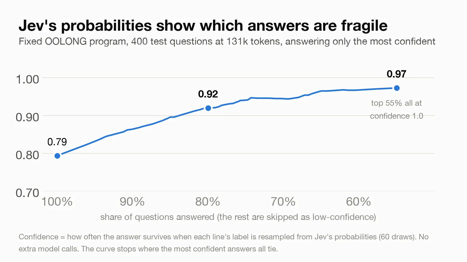
With the fixed OOLONG program and two-order labels, on the 400 questions of the test split at 131k, the 60% of answers with confidence above 0.95 scored 0.97, and the 101 answers at or below 0.5 scored 0.36. Declining to answer the least confident 20% lifts the score on the rest from 0.79 to 0.92. A generative sub-call can give a similar signal only through token log-probabilities, which Claude’s API doesn’t expose, or by running each call several times.

Resampling treats each label’s uncertainty as an independent coin flip, though, and Jev’s mistakes aren’t random. It tends to push the same kinds of items toward the same wrong label, and asking again mostly gives the same label back. So the spread of the resampled counts misses that shared bias, the way weighing yourself multiple times on a miscalibrated scale that reads two pounds heavy only shows you the jitter. In practice, the 90% ranges it implied for counts held the true count only 30% of the time on TREC and 75% on spam. Thus, the confidence is good for deciding which answers to trust, but not for putting error bars on a count.

Escalating uncertain items to a bigger model

The probabilities also say which items are hard. Jev labels everything, and only the items where its top probability falls below a threshold go to Claude Haiku 5.5, playing the slower, more deliberate System 2.

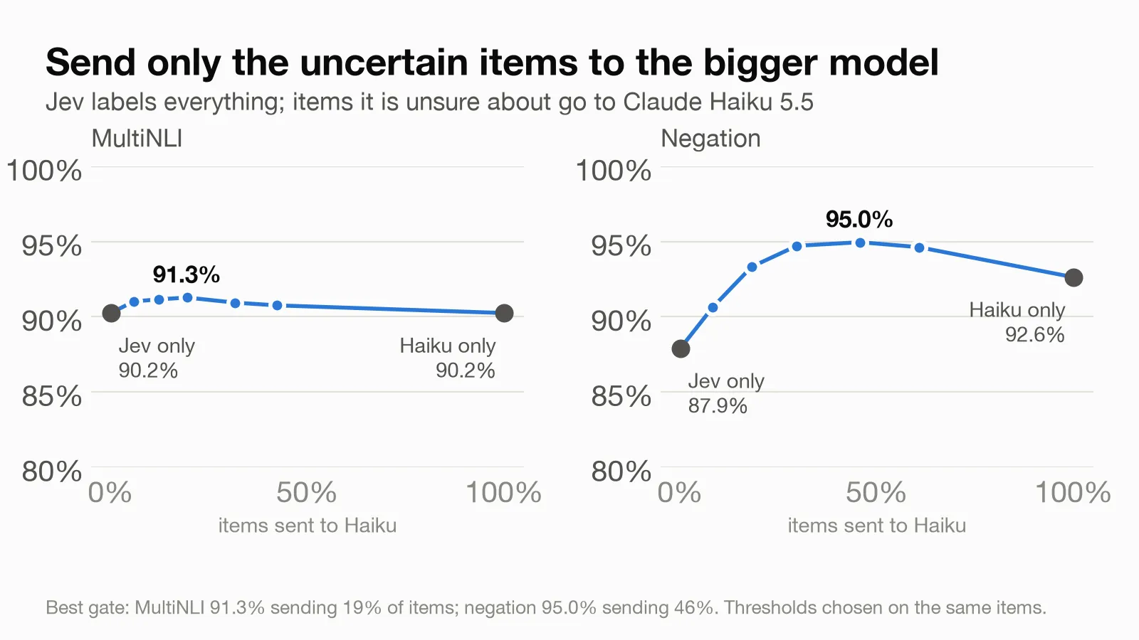
On MultiNLI (does sentence B follow from sentence A?), Jev alone got 89.7% and Haiku alone 90.2% of 3,497 items. Sending Haiku only Jev’s least confident 12% gave 91.5%, higher than either model alone. On a negation dataset (is this single-sentence claim true?), Jev alone got 87.9% and Haiku alone 92.6% of 5,438 items. Sending Haiku the least confident 46% gave 95.0%, again higher than either.

I chose those thresholds after seeing the results on these same items, so the peaks are optimistic. The curves are flat near the top, though, and the neighboring thresholds gave 91.1% and 91.3% on MultiNLI, and 94.7% and 94.8% on negation. On TREC, sending Haiku the 18.6% of items Jev was least sure about raised accuracy from 94.4% to 96.3%.

For the gate to beat both models, Jev and Haiku have to make different mistakes, and Jev’s errors have to cluster in its low-confidence items, and on these datasets both did.

Correcting label bias with six weights

Jev’s mistakes lean in consistent directions. On TREC, for example, it calls some entity questions descriptions. Per item that barely matters, but exact counts over thousands of items add it up. A cheap fix, the same idea as DSPy’s ReAnchor optimizer, is one multiplier per label, fitted on 300 labeled items and applied to the probabilities before taking the top label. On OOLONG’s TREC tasks it cut the per-label count error from 7.9% to 2.6% and raised the score from 0.75 to 0.81, with the 300 fitting items removed from every test context. The gain was in the shorter contexts; at 131k the score went from 0.71 to 0.69.

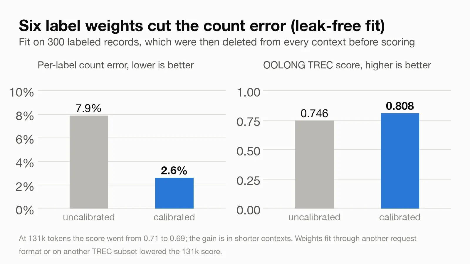
The weights correct Jev’s priors for one dataset and one request format (here 0.1 for descriptions, 0.25 for entities and 2 for people), so fit them on a sample of the data you’ll run on, in the request format you’ll use. Fitted through DSPy’s request format they dropped accuracy to 87% on mine; fitted on TREC questions from outside OOLONG’s slice they lowered the 131k score. With a few hundred labeled examples of your own, it’s a worthwhile tune-up. It pairs especially well with the cheaper format from the Batching section, whose counts start further off. There the same fit cut the count error from 11.4% to 2.2%, and raised the 131k score from 0.69 to 0.81, where with the default format it slipped.

Using it with dspy.RLM

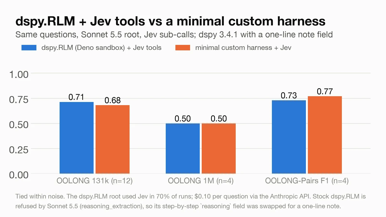
DSPy 3.4 added native Jev support and the ReAnchor optimizer. rlm_tools() returns plain Python functions with docstrings written for the root, so they drop into dspy.RLM(tools=...) unchanged. On the same questions, dspy.RLM (3.4.1, with the note-field change described in Limitations) scored 0.71, 0.50 and 0.73 on OOLONG at 131k, OOLONG at 1M and OOLONG-Pairs, against 0.68, 0.50 and 0.77 for my minimal harness (12, 4 and 4 questions), which is a tie at these sample sizes. Its root chose Jev in 14 of 20 runs, at about $0.10 a question.

Takeaways

It’s easy to say classifiers have always existed (they have), or that there are plenty of ways to get agents and LLMs to manage state outside their own context. But what drew me to the work on RLMs and to Jev is the idea that if we treat them as programming primitives, things a program can call and compose at runtime, the nature of writing software itself might change. My goal here was to explore that space a little, see firsthand where System One models are useful inside an RLM, and start building an intuition for how to use them well. This was a weekend of experiments with small samples, so the results are directional, but here’s what I took away from them.

Where it clearly helped was per-item judgment over a lot of text. Inside an RLM, Jev matched an LLM sub-call from 32k to 1M tokens, and at 1M it cost half as much and ran six times faster. The return type mattered even more. A distribution per item always parses, the roots used the probabilities without being told to, and the same probabilities let a program skip its fragile answers or send only uncertain items to a bigger model.

The case for RLMs over long context held up too. Even with 1M-token windows, Sonnet and Haiku reading everything lost to the RLM at 131k and at 1M.

Where it didn’t help was just as useful to see. At 32k the choice of sub-call barely mattered. The roots in this round often didn’t need help. They deduplicated before calling anything, labeled tiny subsets themselves, and solved BrowseComp-Plus with regex. A sub-call should be cheap and fast enough that the root uses it when it helps and skips it when it doesn’t. A decision model fits that better than a generative one, but on BrowseComp-Plus the root did best with no sub-calls at all. That’s the rule the RLM already follows for parsing and counting: fit the tool to the job. Keep in code whatever code can do, and send a model only the judgments a string match can’t make.

A few practical lessons:

• Put each item in its own question, and never make the model find items by position.
• Batch a few hundred items per request.
• Use the probabilities, not just the top label.
• With a few hundred labeled examples, fit per-label weights. They pair especially well with sending label descriptions once per request.
• Skip sub-calls when a string match will do.

This is a first pass, and I came away more excited than I started. A root that writes code over any amount of text and a sub-call that returns calibrated answers it can compute with fit together well, and there’s a lot left to try: judgments that aren’t classification, deeper recursion, other root models, and new ways of combining the two.

Limitations

• Samples are small. Most settings have 20 questions and some have 3 or 5, and comparisons to the paper’s GPT-5 numbers are sanity checks.
• Jev isn’t perfectly deterministic. Accuracies on hundreds of items move by a few tenths of a point between runs, and fitted label weights amplify that (fits on two TREC samples gave 131k scores of 0.70 and 0.64), so treat the calibration result as a direction.
• About 18% of root turns were lost because Sonnet 5.5 wrapped its Python in tool-call markup, at similar rates in both arms. It contributed to all four OOLONG runs that ran out of turns.
• Under load, Jev throttled well below its documented 80 requests per second. Batching helps, but long passes still needed retries.
• Sonnet 5.5 refuses stock dspy.RLM (reasoning_extraction) because its prompt asks for a step-by-step reasoning field. For the numbers above I replaced that field with a one-sentence note, following Anthropic’s guidance, and reported it upstream (stanfordnlp/dspy#10641). The DSPy team has since merged a fix (#10643), due in the next release. In my test of that fix, stock dspy.RLM ran all 20 questions without a refusal.

Related work

jev-rlm (@sancheznoseke) was the first to put Jev inside an RLM, as a chunk filter on a needle-in-a-haystack task, with one run with Jev and one without. toolJev builds an RLM-style tool router on Jev.

Recursive Decision Models (@raw_works) goes the other way, with decision models at the center, recursing without an LLM. That thread explicitly set aside “giving an LLM agent a decision model as a tool”, which is the combination this post measures.

SubQ Snap, launched October 12, 2026, is a long-context decision model that reads up to 384K tokens. It approaches the problem from the other direction, with one model that reads more. The InfiniteBench result above is a reason for caution there, since a model reading 650k tokens in one go missed questions that the same model got right from the relevant 8,000 words.

---

The runs reported here cost about $7 in Jev usage and about $113 in Claude usage at list price, including $1.95 through the Anthropic API for the dspy.RLM runs and roughly $2 of BrowseComp-Plus grading that wasn’t logged. The code, the raw results and the scripts that reproduce every number are at github.com/jhochenbaum/rlm-jev; uv sync sets everything up.

Acknowledgements

Thanks to Alex Zhang, Tim Kraska and Omar Khattab for RLMs and for a post worth learning from, to the DSPy team for dspy.RLM, and to TypeSafe for Jev. Thanks also to the OOLONG, BrowseComp-Plus and InfiniteBench authors for making their benchmarks available.